
If your returns spiked after introducing BNPL, you’re not alone. Returns are a massive cost center—U.S. retailers saw roughly $685B in returns in 2024, with about 15.14% of those suspected as fraudulent, according to the Appriss Retail & Deloitte 2024 Consumer Returns Report (2024). Industry-wide return volumes also climbed to an estimated $890B in 2024, and ecommerce return rates hover in the high teens, per the NRF and Happy Returns 2024 report (2024). The open question for many operators is causal: did BNPL cause your return rate to surge, or did other factors (seasonality, mix shifts, promotions, fraud) move first?
This article lays out a practitioner-ready workflow to test causality—so you can decide whether to expand, gate, or roll back BNPL with confidence. It draws on standard causal methods (DiD/ITS) and current evidence, including BNPL’s known demand effects from a peer‑reviewed 2024 study that found BNPL can lift purchasing (6.42% in that dataset) for certain segments using a synthetic DiD design, without directly quantifying returns (Journal of Retailing 2024 study on BNPL purchase behavior). We also consider the evolving fraud context, where BNPL is being exploited by synthetic identities and first‑party abuse per the Merchant Risk Council’s 2024 analysis (2024).
What to instrument before you test
From experience, most causality projects succeed or fail in data preparation. Instrument these fields consistently across channels before running models:
- Payment method tags
- BNPL provider (e.g., Affirm/Afterpay/Klarna/PayPal Pay in 4), plan type, installments, approval outcome, transaction ID.
- Provider-level events: disputes opened/closed, refund posted timestamps.
- Order/return lifecycle
- Fulfillment date, delivery confirmation (if available), RMA creation date, return receipt date, refund issue date.
- Cohorting dimensions
- Store/channel, device, geo/market, acquisition source/campaign, new vs repeat customer, tenure, price band, SKU/category.
- Calendar and seasonality
- ISO week, month, holiday flags, major promotions/sale events, known outages or logistics disruptions.
Tip: Create a durable “order cohort date” (e.g., fulfillment week) and analyze outcomes within fixed windows (e.g., returns reported within 60 days of that cohort). This avoids moving-window bias when refund posting lags vary by provider.
Metrics that matter (with definitions)
Use precise, windowed definitions that match your policy and refund SLAs:
- Return rate (order-level): returned_orders / fulfilled_orders, within X days from fulfillment (commonly 45–90 days). Define “returned” as refund issued or return received; be consistent.
- Return rate (unit-level): returned_units / sold_units, within the same X-day window.
- Time-to-return: days from fulfillment to RMA creation or return receipt.
- Return frequency per customer: returns per 100 orders, rolling 90 days.
- Refund cycle time: days from RMA open to refund issued; track “cash exposure days.”
- Margin erosion: (refunds + reverse logistics + restocking + write‑downs + BNPL fees) / net sales, by cohort.
- Adjacent KPIs: conversion rate, AOV, cancellation rate, exchange ratio, fraud flags, chargebacks per 10k orders.
Context: Retail returns are structurally large and seasonal. 2024 had sizable return volumes, so control for holidays and sales cycles to avoid false attribution, as highlighted by the NRF’s 2024 retail returns report (2024).
Choose the right causal design
There’s no single “best” method; pick the design that fits your rollout pattern and data richness.
1) Difference‑in‑Differences (DiD) with staggered adoption
Use when some units (stores, markets, channels, cohorts) get BNPL while others don’t, and you have pre/post data for both. The core assumption is that treated and control units would have followed parallel trends absent BNPL. Modern guidance recommends estimators built for staggered adoption and heterogeneous effects—see Callaway & Sant’Anna’s multi‑period DiD framework (2021) and Sun & Abraham’s event‑study estimator discussed in Cunningham’s Mixtape (updated 2022).
Implementation pattern:
- Outcome(s): return rate (order- and unit-level), time‑to‑return, margin erosion; plus conversion and AOV for trade‑off analysis.
- Treatment: BNPL_available flag at unit‑time (e.g., market‑week).
- Controls: seasonality (week/month dummies), holiday flags, promotions, SKU/category mix, device, traffic source, geo fixed effects.
- Diagnostics: pre‑trend visualization; test “lead” effects in an event‑study—pre‑period leads should be near zero if parallel trends hold. See The Effect Book’s DiD chapter (2025 update) for pragmatic guidance.
Reporting: Use group‑time ATT (average treatment effect on treated) curves to see dynamics (e.g., effect in months 1–6 after BNPL on). Cluster SEs by unit; consider wild bootstrap if few clusters.
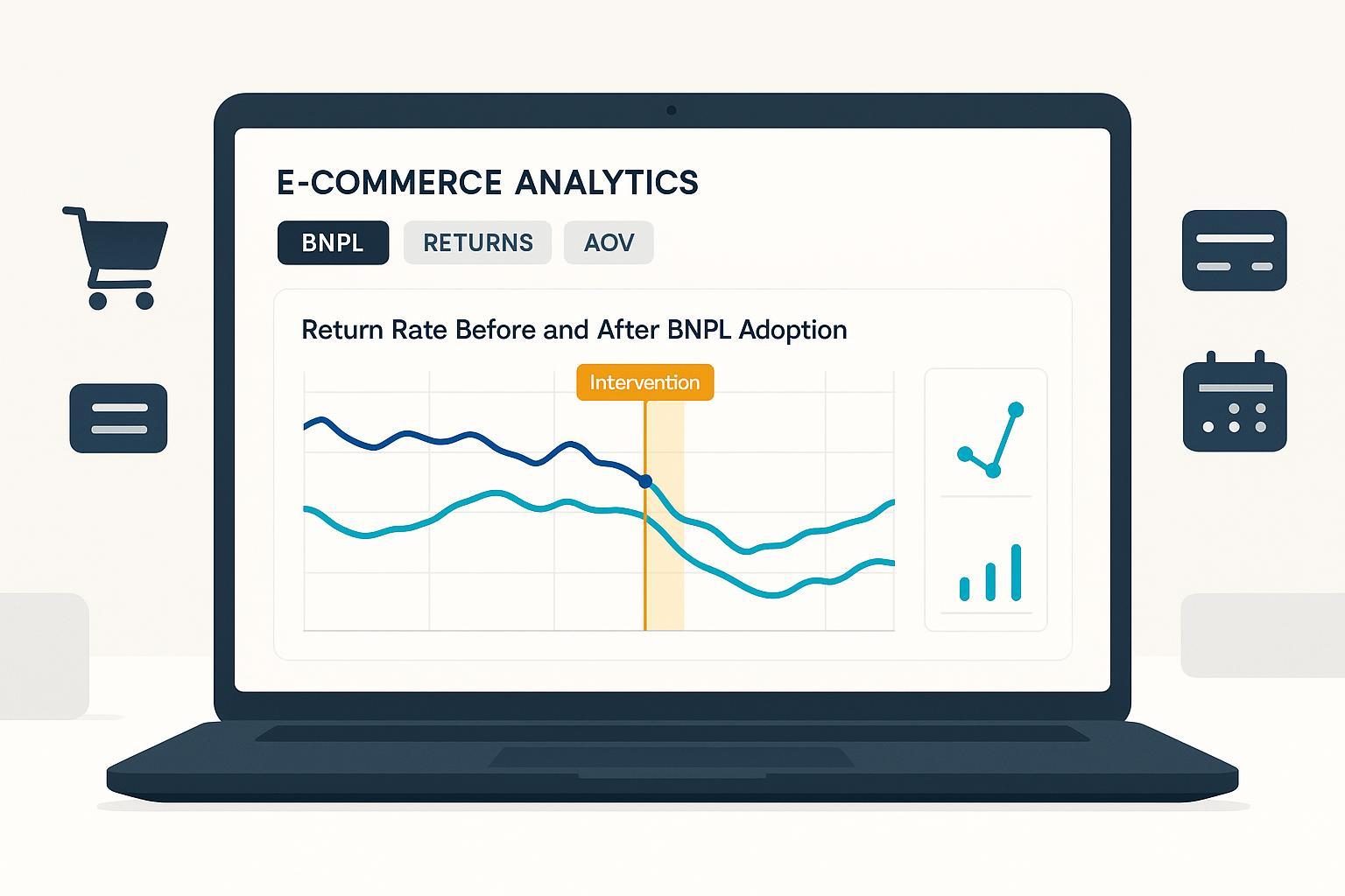
2) Interrupted Time Series (ITS) / Bayesian structural time series (BSTS)
Use when you primarily have a single unit (e.g., one flagship D2C store) with a clear intervention date and long, stable pre‑period. Model seasonality and autocorrelation explicitly via AR terms and calendar dummies. Overviews in health policy evaluation are accessible and applicable, such as Bernal et al., interrupted time series regression (2016). For Bayesian variants and geolift‑style controls, see CausalPy’s ITS notebooks (2025).
Implementation pattern:
- Weekly outcome series for at least 12–18 pre‑weeks; more is better.
- Include exogenous regressors: promotions, marketing spend, category mix, traffic, device share.
- Add a synthetic control if possible (unaffected category/geo), turning ITS into a “controlled ITS.”
- Sensitivity: vary pre/post windows; run placebo dates.
3) Propensity score methods (matching/weighting)
Use when selection into BNPL exposure is non‑random (e.g., mobile users or higher AOV baskets are more likely to use BNPL). Matching or weighting on the propensity to adopt can reduce imbalance; combine with DiD for a matched‑DiD that is robust to observables.
Step‑by‑step workflow to test causality
- Formulate the business hypothesis: “BNPL adoption increased our 60‑day order‑level return rate by ≥X bps after controlling for seasonality, promotions, and mix.”
- Choose units: Identify treated units (BNPL on) and comparable control units (no BNPL), or plan ITS if a single unit.
- Lock the observation windows: Pre‑period of 12–18 weeks; post of at least 8–12 weeks initially (extend to capture lagged returns).
- Finalize outcome definitions: Prefer order‑level return rate with a 60‑day window for first pass; also compute unit‑level and time‑to‑return.
- Validate instrumentation: QA BNPL flags, provider IDs, refund timestamps, and dispute events against settlement files.
- Baseline pre‑trends: Plot pre‑adoption return rates for treated vs control; ensure no major divergence.
- Pick the model: Staggered DiD (Callaway & Sant’Anna / Sun & Abraham) if multiple units; ITS/BSTS if one unit with strong pre‑period.
- Specify controls: Week and month fixed effects, holiday dummies, promo flags, category/device/geo mix, and traffic source.
- Estimate effects: Report ATT with confidence intervals; include dynamic event‑study effects by months since BNPL.
- Run robustness: Placebo leads (should be ~0), alternative controls, drop high‑leverage periods (outages, strikes), try triple difference across categories when mix shifts are large. For diagnostics and negative‑weight pitfalls in TWFE, see Andrew Heiss’s TWFE diagnostics (2021).
- Segment heterogeneity: New vs repeat, category clusters, high‑ vs low‑AOV baskets, mobile vs desktop, geography.
- Incorporate fraud context: Re‑estimate excluding orders with fraud flags and compare to full sample. The Merchant Risk Council’s 2024 fraud overview (2024) underscores first‑party misuse and synthetic ID risks that can bias return metrics.
- Cross‑KPI trade‑offs: Report conversion and AOV changes alongside return rate and margin erosion. BNPL can lift demand—evidence from the 2024 Journal of Retailing BNPL study indicates increased purchasing for certain cohorts—so net margin impact is the decision variable.
- Decide and document: Keep, gate, or roll back BNPL; document model formulae, covariates, windows, and caveats.
Robustness and sensitivity checks you shouldn’t skip
- Parallel trends validation: Event‑study “lead” coefficients should be small and statistically indistinguishable from zero pre‑BNPL. See the Mixtape DiD chapter’s pre‑trend guidance (updated 2022).
- Placebo dates: Assign a fake BNPL start date in the pre‑period; you should estimate no material effect.
- Alternative control groups: Swap in different control markets/channels; check stability of ATT.
- Specification variants: Add/remove covariates; use within‑category models; winsorize outliers.
- SEs and aggregation: Cluster by unit; if few clusters, consider wild bootstrap; aggregate to weekly rates when daily volatility obscures signals.
- Triple difference: If category mix is shifting, difference across categories as a third dimension; background in the Econometrics Journal’s triple difference discussion (2022).
Pilot rollout blueprint (timeline and guardrails)
- Scoping (2–3 weeks)
- Units: Pick 2–4 treated markets/channels and 2–4 controls with similar pre‑trends and mix.
- Metrics: Primary 60‑day order‑level return rate; secondary conversion, AOV, time‑to‑return, margin erosion.
- Data audit: Confirm BNPL tags and refund timestamps; verify campaign and holiday flags.
- Design (1–2 weeks)
- Pre window: 12–18 weeks; Post: 8–12 weeks minimum (extend as needed).
- Methods: Staggered DiD + event‑study; run a parallel ITS for a flagship channel if suitable.
- Power: Compute a back‑of‑envelope minimum detectable effect using historical variance; extend horizon if underpowered.
- Execution (ongoing)
- Change log: Freeze non‑essential payment/policy changes; log promotions and price changes.
- QA: Daily checks for BNPL tagging and refund posting latency; reconcile to provider settlement files.
- Analysis (2 weeks)
- Pre‑trend, placebo, alternative controls, heterogeneity, fraud‑exclusion re‑run.
- Decision memo: Effects, uncertainty, operational implications, and next iteration.
Pitfalls that derailed teams (and how to avoid them)
- Seasonality confounding: Compare like‑for‑like weeks; include holiday dummies and promotional periods, consistent with the elevated holiday return patterns flagged by the NRF 2024 returns research (2024).
- Mix shifts: Run within‑category models or triple difference; ensure category and price‑band controls are in place.
- Refund lag bias: If providers post refunds 5–10 business days after merchant action, align the return window (e.g., 60/90 days) so late postings don’t leak across cohorts.
- Mis‑tagged BNPL orders: Cross‑check against provider settlement/Dispute files; missing provider IDs can scramble treatment flags.
- Fraud spikes: Model with and without fraud‑flagged orders; MRC shows BNPL is a target for synthetic IDs and “buy now, pay never” patterns in 2024 (MRC AtData analysis).
Toolbox: Analytics options for causal testing (parity listing)
- Shopify Analytics — native commerce metrics; export for custom modeling.
- Adobe Commerce BI — enterprise data modeling with dashboards.
- Looker/Looker Studio — semantic modeling and visualization, with SQL-powered analysis.
- WarpDriven — AI‑first ERP/analytics unifying orders, returns, inventory, and payment metadata; supports custom modeling workflows and cohorting at scale. Disclosure: WarpDriven is our product.
(Select based on your need to tag BNPL metadata, run custom DiD/ITS models, cohort by category/geo/device, and access provider events via API.)
Operational guardrails specific to BNPL returns
- Refund and dispute flows: Ensure your RMA system updates the BNPL provider as soon as you accept a return. For PayPal Pay in 4, refunds are processed through standard merchant flows and installments are adjusted by PayPal; disputes can trigger reversals—confirm current terms in the PayPal User Agreement and BNPL merchant guide (2025).
- Cash exposure management: Track “cash exposure days” from RMA open to refund issued; reconcile BNPL fees and any fee reversals retained by providers.
- Customer communication: Clearly state BNPL‑specific return timelines on PDP/checkout; train CX to route BNPL disputes appropriately.
- Policy tuning: If causal results show elevated returns concentrated in certain categories or first‑time buyers, consider gating BNPL to repeat customers or low‑return categories.
Reporting template you can adapt
Standardize what you publish internally so executives get a decision‑ready view:
- Scope summary
- Units, windows, outcomes, covariates, model(s) chosen.
- Pre‑trend diagnostics
- Side‑by‑side pre‑period plots; event‑study leads near zero.
- Main effects
- ATT for return rate (order‑ and unit‑level) with 95% CI; dynamic effects by months since BNPL on.
- Robustness
- Placebo dates, alternative controls, category‑specific models, fraud‑excluded sample.
- Trade‑off panel
- Conversion, AOV, margin erosion; net impact on contribution margin.
- Decision and guardrails
- Keep/gate/roll back; specific policy changes; next monitoring cycle.
Why causality here is non‑optional
BNPL can expand the top of the funnel—peer‑reviewed evidence shows increased purchasing for certain cohorts using synthetic DiD in 2024 (Journal of Retailing BNPL behavior study). But returns and fraud are large, structural realities—2024 saw hundreds of billions in returns and substantial fraud shares, per Appriss & Deloitte’s 2024 returns report and the NRF 2024 returns estimate. The combination demands disciplined causal testing, not intuition.
If you run the workflow above—clean instrumentation, staggered DiD or ITS with strong diagnostics, and a clear trade‑off panel—you’ll have a decision‑grade read on whether BNPL is helping or hurting net margin in your context. Then you can scale with confidence, gate to the right segments, or pivot without second‑guessing.